Paper discussion: The three-species problem: incorporating competitive asymmetry and intransitivity in modern coexistence theory by Ravi Ranjan, Thomas Koffel, Christopher A. Klausmeier. (Link to the paper will be added soon)

Materials

The Mathematica notebook is HERE.

Paper discussion

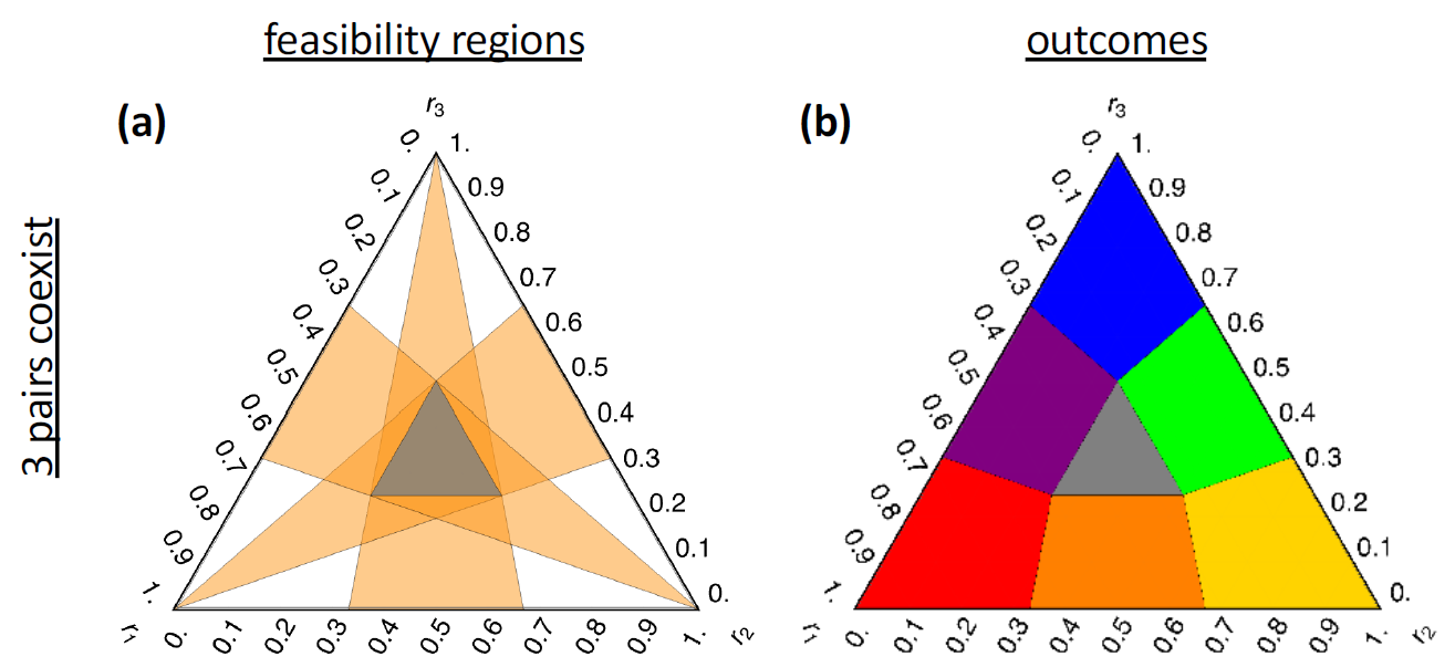
We talked about the three species competition. There are many types of competition outcomes. They are determined by the 12 parameters in the model, i.e., the three intrinsic growth rates and 9 pairwise competition coefficients. The authors showed that the outcome of the competition is associated with the cyclic asymmetry, which is a triplet-wise quantity.

Paper Abstract

While natural communities can contain hundreds of species, modern coexistence theory focuses primarily on species pairs. Alternatively, the structural stability approach considers the feasibility of equilibria, gaining scalability to larger communities but sacrificing information about dynamic stability. Three-species competitive communities are a bridge to more-diverse communities. They display novel phenomena while remaining amenable to mathematical analysis, but remain incompletely understood. Here, we combine these approaches to identify the key quantities that determine the outcome of competition. We show that pairwise niche overlap and fitness differences are insufficient to completely characterize competitive outcomes, which requires a strictly triplet-wise quantity: cyclic asymmetry. Low pairwise niche overlap stabilizes the triplet, while high fitness differences promote competitive exclusion. The effect of cyclic asymmetry on stability is complex and depends on pairwise niche overlap. In summary, we elucidate how pairwise niche overlap, fitness differences, and cyclic asymmetry determine the outcome of three-species competition.

Model

The three-species Lotka-Volterra competition model is defined as

\[ \begin{aligned} \frac{dN_1}{dt} &= \left(r_1 - \alpha_{11} N_1 - \alpha_{12} N_2 - \alpha_{13} N_3\right) N_1 \\ \frac{dN_2}{dt} &= \left(r_2 - \alpha_{21} N_1 - \alpha_{22} N_2 - \alpha_{23} N_3\right) N_2 \\ \frac{dN_3}{dt} &= \left(r_3 - \alpha_{31} N_1 - \alpha_{32} N_2 - \alpha_{33} N_3\right) N_3 \end{aligned} \]

where \(N_1\), \(N_2\) and \(N_3\) are the population sizes of species 1, 2 and 3, respectively, \(r_1\), \(r_2\) and \(r_3\) are the intrinsic growth rates, and \(\alpha_{ij}\)s are the competition coefficients.

The simulation

#| standalone: true
#| viewerHeight: 700
#| viewerWidth: 1000

library(shiny)
library(bslib)
library(plotly)
library(Matrix)

Sim_lotka_volterra <- function(tt, alpha11, alpha12, alpha13, alpha21, alpha22,
                               alpha23, alpha31, alpha32, alpha33, r1, r2, r3, N10, N20, N30) {
  N1 <- c(N10)
  N2 <- c(N20)
  N3 <- c(N30)
  cc <- c(0)
  for(ti in 1:tt){
    dN1 <- (r1 - alpha11 * N1[ti] - alpha12 * N2[ti] - alpha13 * N3[ti]) * N1[ti]
    dN2 <- (r2 - alpha21 * N1[ti] - alpha22 * N2[ti] - alpha23 * N3[ti]) * N2[ti]
    dN3 <- (r3 - alpha31 * N1[ti] - alpha32 * N2[ti] - alpha33 * N3[ti]) * N3[ti]
    N1 <- c(N1, N1[ti] + dN1)
    N2 <- c(N2, N2[ti] + dN2)
    N3 <- c(N3, N3[ti] + dN3)
    cc <- c(cc, ti)
  }
  return(data.frame(N1 = N1, N2 = N2, N3 = N3, cc = cc))
  
}




# Define UI for app that draws a histogram ----
# Define UI for app that draws a histogram ----
ui <- fluidPage(
  headerPanel(''),
  
  fluidRow(
    column(12, 
           tags$head(tags$style("#text{color: black;
                                 font-size: 30px;
                                 font-style: italic;
                                 }"
           )
           ),
           plotlyOutput("plot", width=860)
    )
  ), 
  
  fluidRow(
    column(3, 
           div(style="height: 80px;",sliderInput('r1', 'r1', 1.1, min = 0.1, max = 3)),
           div(style="height: 80px;",sliderInput('r2', 'r2', 1.1, min = 0.1, max = 3)),
           div(style="height: 80px;",sliderInput('r3', 'r3', 1.1, min = 0.1, max = 3))
    ),
    column(3,
           div(style="height: 80px;", sliderInput('alpha11', HTML("&alpha;<sub>11</sub>"), 1.0, min = 0.1, max = 5)),
           div(style="height: 80px;",sliderInput('alpha12', HTML("&alpha;<sub>12</sub>"), 0.15, min = 0.1, max = 5)),
           div(style="height: 80px;",sliderInput('alpha13', HTML("&alpha;<sub>13</sub>"), 1.9, min = 0.1, max = 5))
    ),
    column(3,
           div(style="height: 80px;",sliderInput('alpha21', HTML("&alpha;<sub>21</sub>"), 2, min = 0.1, max = 5)),
           div(style="height: 80px;",sliderInput('alpha22', HTML("&alpha;<sub>22</sub>"), 1.1, min = 0.1, max = 5)),
           div(style="height: 80px;",sliderInput('alpha23', HTML("&alpha;<sub>23</sub>"), 0.2, min = 0.1, max = 5))
    ),
    column(3,
           div(style="height: 80px;",sliderInput('alpha31', HTML("&alpha;<sub>31</sub>"), 0.15, min = 0.1, max = 5)),
           div(style="height: 80px;",sliderInput('alpha32', HTML("&alpha;<sub>32</sub>"), 2.1, min = 0.1, max = 5)),
           div(style="height: 80px;",sliderInput('alpha33', HTML("&alpha;<sub>33</sub>"), 1.2, min = 0.1, max = 5))
    )
  )
  
  
)

server <- function(input, output, session) {
  N1 <- seq(0, 20, 0.01)
  N2_1 <-reactive({
    (input$r1 - input$alpha11 * N1) / input$alpha12 
  })
  
  N3_1 <-reactive({
    (input$r1 - input$alpha11 * N1) / input$alpha13 
  })
  
  N2_2 <- reactive({
    (input$r2 - input$alpha21 * N1) / input$alpha22
  })
  
  
  # sim lv model
  sim_result <- reactive({
    Sim_lotka_volterra(100, input$alpha11, input$alpha12, input$alpha13,
                       input$alpha21, input$alpha22, input$alpha23,
                       input$alpha31, input$alpha32, input$alpha33,
                       input$r1, input$r2, input$r3, 0.1, 0.1, 0.1)
  })
  
  
  output$plot <- renderPlotly({
    Ns <- data.frame(N1 = N1, N2_1 = N2_1(), N2_2 = N2_2())
    pos_Ns <- Ns[Ns$N2_1 >= 0 | Ns$N2_2 >= 0,]
    x_lim <- c(0, max(pos_Ns$N1) + 1)
    y_lim <- c(0, max(pos_Ns$N2_1, pos_Ns$N2_2)+1)
    p <- plot_ly(sim_result(), x = ~N1, y = ~N2, z = ~N3, type = 'scatter3d',  mode = 'lines+markers',
                 line = list(width = 6,  color = ~cc, colorscale = list(c(0,'#BA52ED'), c(100,'#FCB040'))),
                 marker = list(size = 3.5, color = '#56A902'),
                 width = 500, height = 400)
      
    # p <- layout(p, scene = list(xaxis = list(range = c(0, 1.5)), yaxis = list(range = c(0, 2)),
    #                              zaxis = list(range = c(0, 2))))
    
    
    p
  })
  
}
# Create Shiny app ----
shinyApp(ui = ui, server = server)

References

Ravi Ranjan, Thomas Koffel, Christopher A. Klausmeier, The three-species problem: incorporating competitive asymmetry and intransitivity in modern coexistence theory, 2024, in press.